Data Entry

Text Editing

Data that you type in a worksheet is in fact entered in cells, except when you are drawing. To use Microsoft Excel with more finesse, you should familiarize with cells, their functionality, their configuration, and their relationships with each other and with the whole software.

The primary technique you can use to get acquainted with the software is by entering data, primarily text, then manipulate various components of your application in order to customize it.

Unlike a traditional word processor, Microsoft Excel has a unique way of treating text and considering any data you type in a cell. You should be aware of the default settings that the software acts on when you type data, how it considers and treats various numbers, dates, and currency values, etc.

We have already seen how to do basic data entry into cells. The entries we used so far were short expressions consisting of one word, we need to find out whether a cell can accept text that is wider than the displayed width, if so, what happens if text goes "overboard"?
We know that data entered in a cell is confined to that cell. If you type text that is longer than the cell's width, the content will display fine, giving the impression that the text is covering more than one cell or that the cell on the right side is no more available. Data you type is always in its cell. If you type anything in a cell, its content will take priority in displaying its content; therefore the content of the left cell will appear cut. That's why you should be very familiar with the way a cell (any cell) displays its data, and how every cell relates to the others.

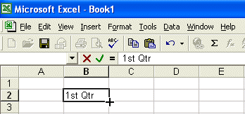
Practical Learning: Entering Text Into Cells

1. To start a new workbook, press Ctrl + N
2. Click cell C2 and type GRIER SUMMER CAMP
3. Click cell B5 and type Employment Application
4. Click cell F5 and type Today:
5. Click cell B8 and type First Name:
6. Press Enter
7. In cell B9, type Address:
8. Press Enter.
9. In cell B10, type City:
10. Press Tab twice.
11. In cell D10, type State:
12. Press Tab twice.
13. In cell F10, type ZIP Code:
14. Click cell B12 and type Nickname:
15. Click cell B13 and type Home Phone:
16. Press Enter.
17. In cell B14, type How Did You Hear About Us?
18. Press Enter.
19. In cell B15, type Position Desired:
20. Press Space 14 times, and type 1)
21. Press Enter.
22. In cell B16, type Desired Hourly Salary:
23. Press Enter.
24. In cell B17, type Starting Date Available:
25. Press Enter
26. In cell B18, type Available Time:
27. Click cell F18 and type E-Mail:
28. Click cell B19 and type Sunday
29. Click cell B21 and type Do You Own Transportation?
30. Click cell C25 and type Employment References And Records
31. Press Enter.
32. Click cell B27 and type Professional References
33. Press Enter.
34. In cell B28, type Please list 3 professional references who can verify your work history and performance.
35. Press Enter.
36. In cell B29, type References should not be relatives and at least two must have directly supervised you.
37. Press Enter.
38. In cell B30, type at some time in your work history.
39. Click cell B32 and type '1.
40. Press Tab.
41. In cell C32, type Name of Supervisor:
42. Click cell G32 and type Title:
43. Click cell C33 and type Company Name And Address:
44. Click cell C35 and type Company Phone Number Including Area Code And Extension:
45. To save the workbook, on the main menu, click File -> Save.
46. Since the workbook has not yet been saved, the File -> Save menu called the Save As dialog box.
    Type GCS Employment Application. If the Save In combo box doesn't display MS Excel Exercises, click the arrow of the Save In combo box and locate the My Documents\MS Excel Exercises folder.
47. After making sure that the MS Excel Exercises folder displays in the Save In combo box, click the Save button.

Techniques Of Cutting and Copying Cells Contents

If you have done word processing before, you are probably familiar with techniques of cutting, copying, pasting, and/or moving text from one part of a document to another, or from one document to another. Although these techniques are available here, Microsoft Excel doesn't quite imitate a word processor. Again, spending time with the software will increase your experience.

When you copy or cut something, it goes in a temporary storage area where it will wait for you to send it somewhere else, an action called pasting. The storage area where the cut or copied data is sent is called the clipboard. In Microsoft Excel 97, you can store only one item at a time in the clipboard. If you cut or copy something, it will replace the content of the clipboard with the new selection. In Microsoft Excel 2000, the clipboard can contain up to twelve items. When the Clipboard toolbar is functional, you can select copied or cut items from its list of buttons. If you use more than 12 stored items, the toolbar functions on a first-in first-out basis.

The Clipboard toolbar can be moved to any location of your choice on the screen. You can also hide/close it if you don't need its services. For this exercise, when the Clipboard toolbar appears, don't close it. Even if you are not preparing for the MOUS exam, you should learn to take advantage of the new clipboard. In case you are not aware, you can use the same Clipboard toolbar in different applications; for example, you can have Microsoft Excel, Microsoft Access, Microsoft Word, and Microsoft Outlook all of them opened at the same time and sharing the same clipboard items. 

Practical Learning: Cutting and Copying Cells Contents

1. To open a new workbook, from the main menu, click File -> Open...
2. Click GCS Employment Application1 and click Open
3. Click cell D8, type MI: and press Enter (the MI stands for Middle Initial)
4. Right-click cell B8 and click Copy from the shortcut menu
5. Click cell F8 and press Enter. That pastes First Name to cell F8
6. Right-click cell B13 and click Copy. At this time, the Clipboard toolbar should be displaying on the screen. If you don't see it, on the main menu, click View -> Toolbars, and click Clipboard. The clipboard toolbar is new to Microsoft Office 2000
7. Click cell F13. You can check what items are on the clipboard any time. Position your mouse on the first button on the clipboard (don't click), a tool tip will appear. Move the mouse to another item and read the tool tip. On the Clipboard toolbar, position the mouse on the last copied item and it should display Home Phone
    
   
   Therefore, click that button
8. Click cell F15 and type 2)
9. Right-click cell F18 and click Cut. One more item gets copied to the Microsoft Office 2000 Clipboard
10. Click cell D12
    On the Clipboard toolbar, position the mouse on the last button on the Clipboard toolbar until you see E-Mail in the tool tip, then click it
11. Select cells from B32:G35
    On the Clipboard toolbar, click the Copy button . That action copies the selected range on the Clipboard. To check that the range of cells has been copied to the Clipboard toolbar, position your mouse on the most recent button on the Clipboard toolbar and read the tool tip
     
    
12. Click cell B38
13. On the Clipboard toolbar, click the last button to paste the copied selection. If you are using Microsoft Excel 97, press Ctrl+V
14. Select cells C38:G41. Position your mouse on the upper border of the selected cells until the mouse pointer turns into a top left pointing arrow
15. Press and hold Ctrl
16. With the mouse pointer still pointing to North West and the mouse now having a small + sign, click and hold the mouse down, then drag towards the lower side of the screen. A small yellowish box guides you to know where the selection is leading
     
    
17. When you get to B44:G47, release the mouse, then release Ctrl
18. To save the workbook, on the Standard toolbar, click the Save button

Text in Cells

Editing cells content consists of deleting, replacing, altering, or adding something in them. You already know that if you click a cell and start typing, its content will be replaced with the new entry. If you want to add or subtract something to a cell's content, you can double-click it; this puts the cell in Edit mode and you can then proceed. An alternative is to give focus to a cell, then press F2, this also puts the cell in Edit mode; this time, the cursor is at the end of the text in the cell; then you can proceed. Whatever technique you use, when you have finished editing a cell, make sure you lose its focus by pressing Tab, Enter, or clicking somewhere else. When you are in Edit mode, the arrow keys are not working, and many actions are not available.

Practical Learning: Editing Text in Cells

1. Click the Sheet2 tab.
2. Double-click cell F8, press Home, press Delete three time, and type La
   Now cell F8 displays Last Name.
3. Click cell F13. In the Formula Bar, double-click Home and type Work
4. Click cell B38 and type '2.
5. Click cell B44 and type '3.
6. Click cell B27, press Ctrl + C
7. Click cell B51 and press Enter
8. Press F2 to initiate editing. Edit the content of cell B51 to display Personal References
9. Click cell B52 and type Please list 2 personal references (must not be a relative)
10. Click cell B54 and type '1.
11. Press Tab and type Name and Address:
12. Click cell C56 and type Phone Number:
13. Press Enter.
14. In cell C57, type Years Acquainted:
15. In cell F57, type Occupation:
16. Press Enter
17. In cell C58, type Natural Relationship:
     
    
18. Save the workbook
19. To close it, press Ctrl+F4

Exploring Cells Content

Introduction

Microsoft Excel shares a lot of characteristics with window applications: the ability to search through the document for a particular word or phrase, the ability to find a word or group of words and replace it with another word or expression.

A feature unique to Microsoft Excel as a spreadsheet application is the ability to fill out some cells with values that belong to a common series. 

Overview of AutoFill

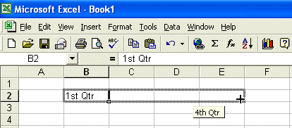
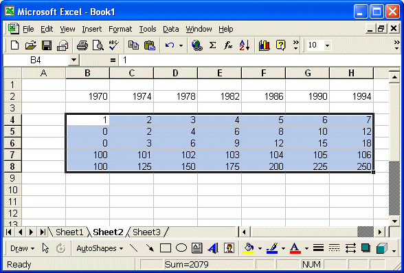
Microsoft Excel recognizes series of items so far as they can be clearly identified, either by the common language or by defining them explicitly in a worksheet. Common series include time, dates, weekdays, or months. Whenever Microsoft Excel can identify the content of a cell as being a series, you can use the Fill Handle to copy adjacent values of the series to neighbor cells. If a series is not obvious, you need to clearly define it so the application can recognize the allure you want to use for the series.

To use the AutoFill, first select a cell or the cells that define the series. Position your mouse on the lower right corner of the selected cell or cells, and then drag in the appropriate direction.

Practical Learning: Exploring the AutoFill

1. In Microsoft Excel, press Ctrl + N to start a new empty workbook.
2. In cell B2, type 1st Qtr
3. Position your mouse on the lower right corner of the selected cell, on the squared point. This point is called the Fill Handle. Your mouse will turn into a +
    
4. Click on the Fill Handle, hold the mouse down and drag in the right direction until you get to cell E2
    
5. Release the mouse. Now you get 1st Qtr, 2nd Qtr, 3rd Qtr, and 4th Qtr.
6. In cell B4, type 1st Grade
7. Drag the Fill Handle in the right direction until you get to cell G4. Then release the mouse to see the subsequent grades.
8. In cell B6, type 1:00
9. Drag the Fill Handle in the right direction until you get to cell H6. Then release the mouse to see the hours displayed.
10. In cell B8, type 9:00 and drag its Fill Handle to cell H8. Notice how Microsoft Excel displays time values in subsequent cells.
11. Click cell B8 and notice the value displayed in the Formula Bar.
12. In cell B10, type 13:00 and drag its Fill Handle to H10. Notice how times get displayed in the other cells.
13. In cell B12, type 9:00 AM and drag its Fill Handle to cell H12. Notice how this time, unlike row 8, Microsoft Excel changed the AM to PM after 11:00 AM:
     
14. In cell B14, type Jan and drag its Fill Handle to cell H14. Notice how the application displays months in subsequent cells
15. In cell B16, type Monday and drag its Fill Handle to cell H16. The computer displays all weekdays
16. In cell B18, type 02/24/1990 and drag its Fill Handle to cell H18. Dates incrementing each day by 1 are displaying in the other cells
17. Click the Sheet2 tab
18. Sometimes Microsoft Excel will not recognize a series with just one value, this happens when the series is not obvious. For example, if you type 1970 in a cell and drag the Fill Handle, the computer would not know whether you want to increment the number by 1, 2, 4, or 10. So you have to specify how the series will be applied. To define a series, type the beginning value, then in the subsequent cell type the incremental values or the value that will be used to define the series.
    In cell B2, type 1970, press Tab
19. In cell C2, type 1974
20. Select cells B2:C2
21. Position the mouse on the Fill handle, which is on the lower right border of cell C2 (because both cells are selected). When the mouse becomes a +, drag the Fill Handle in the right direction up to cell H2. The cell values have been incremented by 1 starting on cell B2
22. In cell B4, type 1
23. In cell C4, type 2
24. In cell B5, type 0
25. In cell C5, type 2
26. In cell B6, type 0
27. In cell C6, type 3
28. In cell B7, type 100
29. In cell C7, type 101
30. In cell B8, type 100
31. In cell C8, type 125
32. Select cells B4:C8
33. Position your mouse on the Fill Handle in the lower right corner of the selected cells (in cell C8). Then drag the Fill Handle to column H and release the mouse:
     
34. Notice that Microsoft Excel could figure out how to handle each series. The first was to increment numbers by 1 starting at 1. The second was asked to list even numbers starting at 0. The third gave a list of odd numbers starting at 0. The third had to count by 1 starting at 100. The fourth was going to find quarter values in a 100 number basis starting at 100
35. In cell B10, type Jan
36. In cell C10, type Apr
37. Select cells B10:C10. Drag the Fill Handle of the selected cells to cell E10. You get the first month on every quarter
38. In cell B12, type 1st Qtr
39. In cell A13, type Jan and drag the Fill Handle of cell A13 to cell C13. That will display the months of the first quarter
40. Select cells A12:C13. Drag the Fill Handle of the selected cells to cell L13
41. Save the workbook as Fill Effects

AutoFill Application

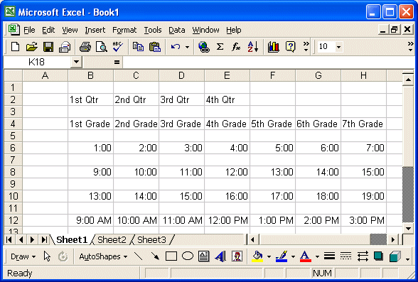
As the AutoFill features provides a quick means of completing cells that can host series data, this feature can be applied in various scenarios.

When creating time sheets, use the weekdays and time periods to complete adjacent cells. In a yearly sales report, Microsoft Excel can recognize series such as months, quarters, and years. In a school’s spreadsheet used to collect students’ grades, a series can be created from 1st Grade, and then dragging the Fill Handle, Microsoft Excel will complete other cells with subsequent class grades.

Practical Learning: Applying the AutoFill

1. On the main menu, click Window.
2. From the list of workbooks, select GCS Employment Application2.
3. Click cell B19.
4. Position the mouse on the lower right corner of the selected cell, on the point, until the mouse pointer becomes a + sign. Click and hold your mouse down, then drag in the right direction to cell H19. That will update the weekdays.
5. Select cells B32:G37
6. Drag the Fill Handle down until the lower border aligns with the lower border of row 48 and release the mouse.
7. In cell B38, type '2.
8. In cell B44, type '3.
9. Select cells B54:F60. Position your mouse on the Fill Handle of the selection. Click and drag down until the lower border of the box you are dragging aligns with row 65, then release your mouse.
10. In cell B61, type '2.
11. Click cell C70 and type Applicant’s Signature:
12. Click cell F70 and type Date:
13. Save and close the workbook (not Microsoft Excel).

Data Entry and Text Management

The GoTo, Find, and Replace Dialog Boxes

To locate a particular cell in Microsoft Excel, you can use the Go To dialog box. This dialog box recognizes cells names by applying the same conventions used by Microsoft Excel. You can get the Go To dialog box from the main menu under Edit.

The shortcuts to access the Go To dialog box are Ctrl + G or F5.

The Find dialog box allows you to find a word in your worksheet, either to simply locate a particular word or multiple instances of a word, or to manipulate a word or groups of words at will.

The Replace dialog box allows you to find a word or group of words and to replace it with a new word or group of words. Both dialog boxes are available from the main menu under Edit.

The shortcut for the Find dialog box is Ctrl + F.

The shortcut for the Replace dialog box is Ctrl + H.

Practical Learning: Finding and/or Replacing Cells Content

1. The GCS Employment Application2 workbook should still be opened.
2. To locate a cell, on the main menu, click Edit -> Go To...
3. Type F13 and click OK.
4. Press Ctrl + G, that calls the Go To dialog box.
5. Type C2 and press Enter.
6. To find a word in the document, on the main menu, click Edit -> Find...
7. In the Find What box, type name and click the Find Next button 8 times. Press Esc to dismiss the Find dialog box.
8. To find a word and replace it with another word, on the main menu, click Edit -> Replace...
9. In the Replace dialog box, in the Find What box, type natural and press Tab. In the Replace With box, type Nature of
    
10. Click Find Next.
11. When the first instance of natural is found, click Replace. Click Replace All.
12. When all instances have been found and replaced, a message box will let you know that Microsoft Excel Cannot Find A Match.
13. Click OK on the message box.
14. Click Close on the Replace dialog box.
15. Press Ctrl + S to save the workbook.

Check Spelling

Although Microsoft Excel is not a word processor, since you can use it to create text documents such as employment applications, brochures, time sheets, etc, it can help you correct typing mistakes of various kinds. It is a good idea to check spelling mistakes in your document before printing it or sending it for an important business transaction. The check spelling is done with the help of a Spelling dialog box that will take you step by step to every word that is questionable. Also, the computer will point out some suggested words that you can use instead of the one at fault.

You can check your worksheet's spelling during or after editing, though the latter is better. To check your document, click the Spelling button on the Standard toolbar or on the main menu, click Tools -> Spelling... The shortcut to access the Spelling dialog is F7. 

Practical Learning: Proof Reading the Worksheet

1. Open the GCS Employment Application3.
2. On the main menu, click Tools -> Spelling...
3. From the Spelling dialog box, the first suggestion is to change the word Employement. After making sure that Employment is selected in the Spelling dialog, then click Change.
4. The next mistake is in the spelling of the word Salary. After making sure that Salary is selected in the dialog, click Change:
    
5. The next problem is with the word Transportation. From the Spelling dialog box, in the list of suggested words, click Transportation and click Change.
6. Accept to Change the word References in cell B27.
7. In cell B28, accept to change performance.
8. In cell B30, accept to change the mistake with history.
9. When the dialog gets to the content of cell B50, select the word personal instead of personnel to replace personel. Then click Replace.
10. Also, correct references.
11. The last problem is with the word sinature. Accept to change it to Signature.
12. After the last problem, Microsoft Excel displays a message box asking whether you want to continue checking at the beginning of the sheet. Click Yes. Another message box should tell you "The spelling check is complete for the entire sheet." Click OK.
13. Press Ctrl + Home to get to the beginning of the worksheet.
14. Press Ctrl + S to save the workbook.